Practical Stability of a Windowed Audio Streaming Buffer

Motivation

Introduction:

Real-time data streaming over Wi-Fi requires client-side buffering to handle network jitter. Many commercial IoT devices specify minimum network requirements (e.g., bandwidth, latency thresholds) to ensure adequate streaming capacity — examples include Google Nest Cam Indoor and Ring Wired Doorbell Pro.

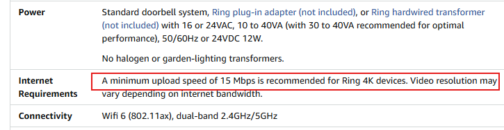
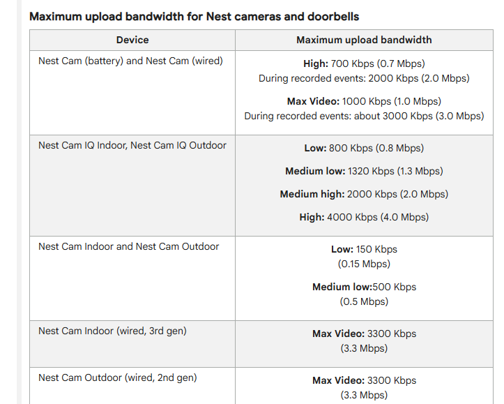
These devices rely on buffers to accommodate temporary network congestion, requiring drain rate > fill rate to prevent overflow. However, sometimes the buffer size is an issue. There is not a lot of free memory left for resource-constrained devices like the ESP32. And that motivates me to find out what is a range of buffer size that is reasonably safe to use, given the network conditions.

Purpose:

In this project, I want to model the buffer filling level of an ESP32 audio streaming system as a stochastic hybrid dynamical system \(\mathcal{H}\) with a continuous flow of filling and discrete stochastic draining jumps. Then I want to prove the practical stability of the buffer level.

There are two parts in this project:

Part 1: I will treat the Round Trip Time (RTT) of the network as a bounded random variable (disturbance), and I want to prove that the buffer level at every jump instant is uniformly globally practically stable (UGpS) in a neighborhood of \(b^* = r_{in} \mu + C_s\) with a tolerance of \(\varepsilon = r_{in} \delta\), where \(\mu\) is the mean of the RTT, \(\delta\) is the bound of the RTT, \(r_{in}\) is the buffer filling rate, and \(C_s\) is the chunk size.

Part 2: Instead of treating the RTT as a bounded random disturbance, I will do some MATLAB simulations to show the distribution of the buffer level at jump instants under different RTT distributions, such as uniform, normal, and exponential distributions.

The Problem

I want to answer the question:

Given that the network condition, of any distribution, is bounded in RTT (round trip time), and assuming that the encoding and decoding process is lossless, and the buffer fill rate is constant, then, in the long run, is the buffer size bounded, and can we characterize the buffer size distribution so we can say that a certain max buffer size is safe?

The System and the Model

System Architecture

The ESP32 audio streaming system runs two asynchronous tasks:

Recording Task: A microphone (INMP441) continuously captures audio and accumulates it into chunks. After recording for a fixed duration \(T_p\), the task pushes a chunk of size \(C_s = r_\text{in} \times T_p\) into a conn queue, where \(r_\text{in}\) is the recording bitrate. (Note: In practice, chunk size may vary slightly due to discrete DMA transfers, though we assume constant size for this analysis.)

Network Task: At every periodic \(T_\text{p}\), this task dequeues a chunk from the conn queue, copying it into the main buffer (which is a hashset so it supports out-of-order arrivals). the send to the server. The buffer only removes a chunk when an acknowledgment arrives from the server. Two hard limits apply:

• Buffer capacity: \(B_\text{max}\) — excess chunks are dropped

• Timeout: \(T_\text{max}\) — chunks not acknowledged within this window are discarded

The Hybrid System Model

This hybrid system model is inspired by the TCP congestion control models in [1] and [2].

Consider the following Stochastic Hybrid System for the audio streaming process:

\[ \begin{aligned} (b, \tau) \in [0, B_{max}] \times [0, \infty), \quad &\begin{cases} \dot{b} = r_\text{in} &\text{if } b < B_{max}\\ \dot{b} = 0 &\text{if } b = B_{max}\\ \dot{\tau} = -1 \end{cases} \\ (b, \tau) \in [C_s, B_{max}] \times \{0\}, \quad &\begin{cases} b^+ = b - C_s \\ \tau^+ = v_j \end{cases} \end{aligned} \]

where

\(v_j > 0\) is the time until the next chunk eviction event. The jump will require at least \(b \geq C_s\) to occur.

and given the conditions:

1. \(C_s = r_{in} \times T_p\).
2. Each chunk's RTT ([3]) is bounded: \(RTT_i \in [\mu - \delta, \mu + \delta]\).
3. \(B_{max} \geq b^* + \varepsilon\), where \(b^*\) is the target buffer size, and \(\varepsilon\) is the tolerance for the buffer size. The \(B_{max}\) is a hardware buffer limit.

We want to prove that:

Define the target buffer size \(b^* \coloneqq r_{in} \mu + C_s\), and the practical neighborhood:

\[ \mathcal{A}_\varepsilon = \{(b, \tau) : |b - b^*| \leq \varepsilon, (b, \tau) \in C \cup D\}, \quad \varepsilon \coloneqq r_{in}\delta\]

let \(\{b_j\}_{j \in \mathbb{N}}\) be the sequence of pre-drain buffer levels that is sampled immediately before jump instants (essentially from a Poincaré Map), I want to show that \(|b_j - b^*| \leq \varepsilon\) for all \(j \in \mathbb{N}\), and therefore it is uniformly globally practically stable (UGpS) of the jump chain on \(\mathcal{A}_\varepsilon\).

Poincaré Map Proof [1] [3]

Instead of analyzing the continuous-time trajectory \((b(t), \tau(t))\) that contains the stochastic timer resets, I sampled at the jump instants \(t_j\), and analyze the discrete sequence \(\{b_j\}\).

The Poincaré Section is the Jump set \(D = \{(b, \tau) : b \geq C_s, \tau = 0\}\), and it captures the full behavior of the trajectory because

1. The trajectory will hit the jump set repeatedly: since the \(\tau\) is reset to a finite value \(v_j\) at every jump, and it's decreasing at a constant rate, it will always hit the jump set again after a finite time.
2. The trajectory will never reach the deadlock zone: It will never reach \(b < C_s, \tau = 0\). The timer was set to \(v_j\) which is the time until the next ACK arrives for a chunk that is already in the hashset buffer. Since flow does not decrease the buffer level, the buffer level will never drop below \(C_s\) when \(\tau = 0\), therefore it will never reach the deadlock zone.
3. The trajectory during the jumps is bounded: since the buffer level is increasing at a constant rate, and the inter-jump timer \(v_j\) is also bounded, the buffer level during the jumps are also bounded.

Since (P1) every solution jumps infinitely often, (P2) no solution terminates, and (P3) inter-jump excursions are bounded, the Poincaré jump map is valid.

Solution

The Arrival Times of the ACKs

Assume that a chunk is sent at time \(k T_p\), its acknowledgment will arrive at time \(a_k = k T_p + RTT_k\).

Since the \(RTT_i \in [\mu - \delta, \mu + \delta]\), the \(a_k\) is also bounded:

\[ k T_p + \mu - \delta \leq a_k \leq k T_p + \mu + \delta \]

Order the \(a_k\) in ascending order, define \(t_j\) to be the \(j\)-th smallest \(a_k\), which are the jump instants of the hybrid system \(\mathcal{H}\).

By definition, the inter-jump timer is therefore \(v_j = t_{j+1} - t_j\).

Proof for the boundary of \(t_j\) and \(v_j\)

Suppose that the first \(c\) chunks' arrival times are \(a_1, a_2, \dots, a_c\). After ordering ascendingly, let \(i\) be the index such that \(i \in \{1, 2, \dots, c\}\), therefore \(a_i \leq i T_p + \mu + \delta\).

Since \(i \leq c\), \(a_i \leq c T_p + \mu + \delta\). Since this holds for every \(i \in \{1, 2, \dots, c\}\), set \(c = j\), therefore \(t_j \leq j T_p + \mu + \delta\).

Similarly, the lower bound of \(t_j\) is \(t_j \geq j T_p + \mu - \delta\).

Therefore, \(j T_p + \mu - \delta \leq t_j \leq j T_p + \mu + \delta\).

Note: Here I bounded the out-of-order arrival time by their arriving index so I don't care when it is being sent (or the \(k\) in the \(a_k\)).

Since \(v_j = t_{j+1} - t_j\).

Lower bound of \(v_j\):

Since \(t_{j+1} \geq (j + 1) T_p + \mu - \delta\) and \(t_j \leq j T_p + \mu + \delta\), the lower bound of \(v_j\) is therefore \(v_j \geq (j + 1) T_p + \mu - \delta - (j T_p + \mu + \delta) = T_p - 2\delta\).

Upper bound of \(v_j\):

Since \(t_{j+1} \leq (j + 1) T_p + \mu + \delta\) and \(t_j \geq j T_p + \mu - \delta\), the upper bound of \(v_j\) is therefore \(v_j \leq (j + 1) T_p + \mu + \delta - (j T_p + \mu - \delta) = T_p + 2\delta\).

Therefore, \(\max(0, T_p - 2\delta) \leq v_j \leq T_p + 2\delta\). Because \(v_j \geq 0\) by definition.

Proof for the boundary of \(b_j\)

At time \(t_j\), there are already \(j - 1\) chunks drained from the buffer. Therefore the buffer level before draining is:

\[ b_j = r_{in} t_j - (j - 1) C_s \]

When at equilibrium, \(RTT_k = \mu\), then \(a_j = t_j = jT_p + \mu\):

\[ b^* = r_{in} (jT_p + \mu) - (j - 1) C_s \\ = r_{in} j T_p + r_{in} \mu - j C_s + C_s \\ = C_s j + r_{in} \mu - j C_s + C_s \\ = r_{in} \mu + C_s \]

The practical neighborhood of \(b_j\) is defined as:

\[ \mathcal{A}_\varepsilon = \{b_j : |b_j - b^*| \leq \varepsilon\} \]

\[ b_j - b^* = r_{in} t_j - (j - 1) C_s - (C_s + r_{in} \mu) \\ = r_{in} t_j - j C_s + C_s - C_s - r_{in} \mu \\ = r_{in} t_j - j C_s - r_{in} \mu \\ = r_{in} t_j - r_{in} j T_p - r_{in} \mu \\ = r_{in} (t_j - j T_p - \mu) \]

From previous, we know that

\[ j T_p + \mu - \delta \leq t_j \leq j T_p + \mu + \delta \\ - \delta \leq t_j - j T_p - \mu \leq \delta \\ - r_{in} \delta \leq r_{in} (t_j - j T_p - \mu) \leq r_{in} \delta \]

Therefore, \(|b_j - b^*| \leq \varepsilon = r_{in} \delta, \quad \forall j \in \mathbb{N}\)

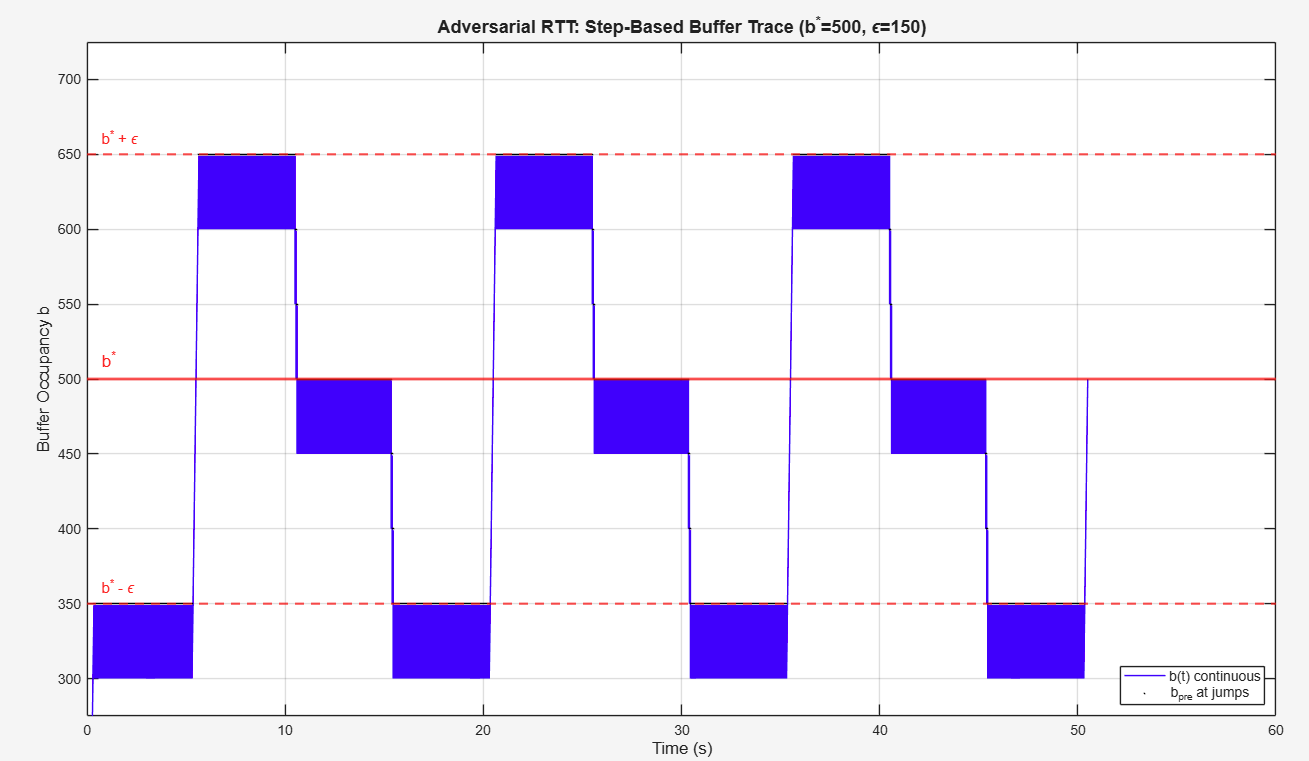
Between jumps, the buffer fills for \(v_j\) seconds. Although \(v_j\) can be as large as \(T_p + 2\delta\), this maximum only occurs when \(b_j\) is near the bottom of the fence (\(b^* - \varepsilon\)) (prove by simulation). Conversely, when \(b_j\) is near the top (\(b^* + \varepsilon\)), \(v_j\) is at most \(T_p\). In both cases, the continuous trajectory peaks at \(b^* + \varepsilon\), never exceeding the pre-drain fence.

Simulation Result

The Random Distribution Case

In the first simulation, the RTT is randomly generated in the range of \([\mu - \delta, \mu + \delta]\), and the buffer level is sampled at the jump instants:

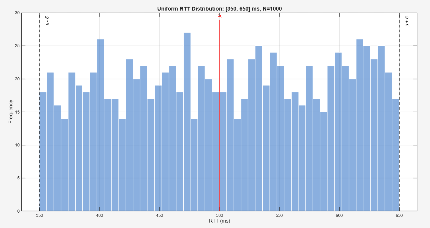
It shows the distribution of RTT is uniform.

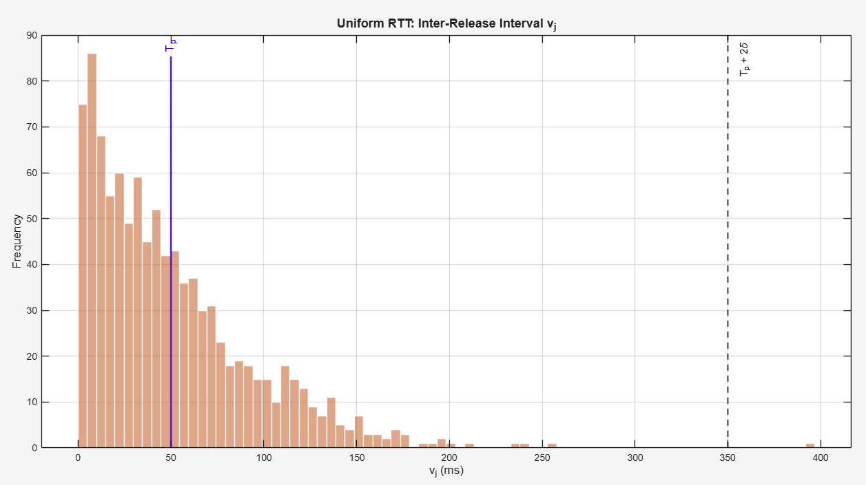
The distribution of the inter-jump timer \(v_j\) is approximately exponential.

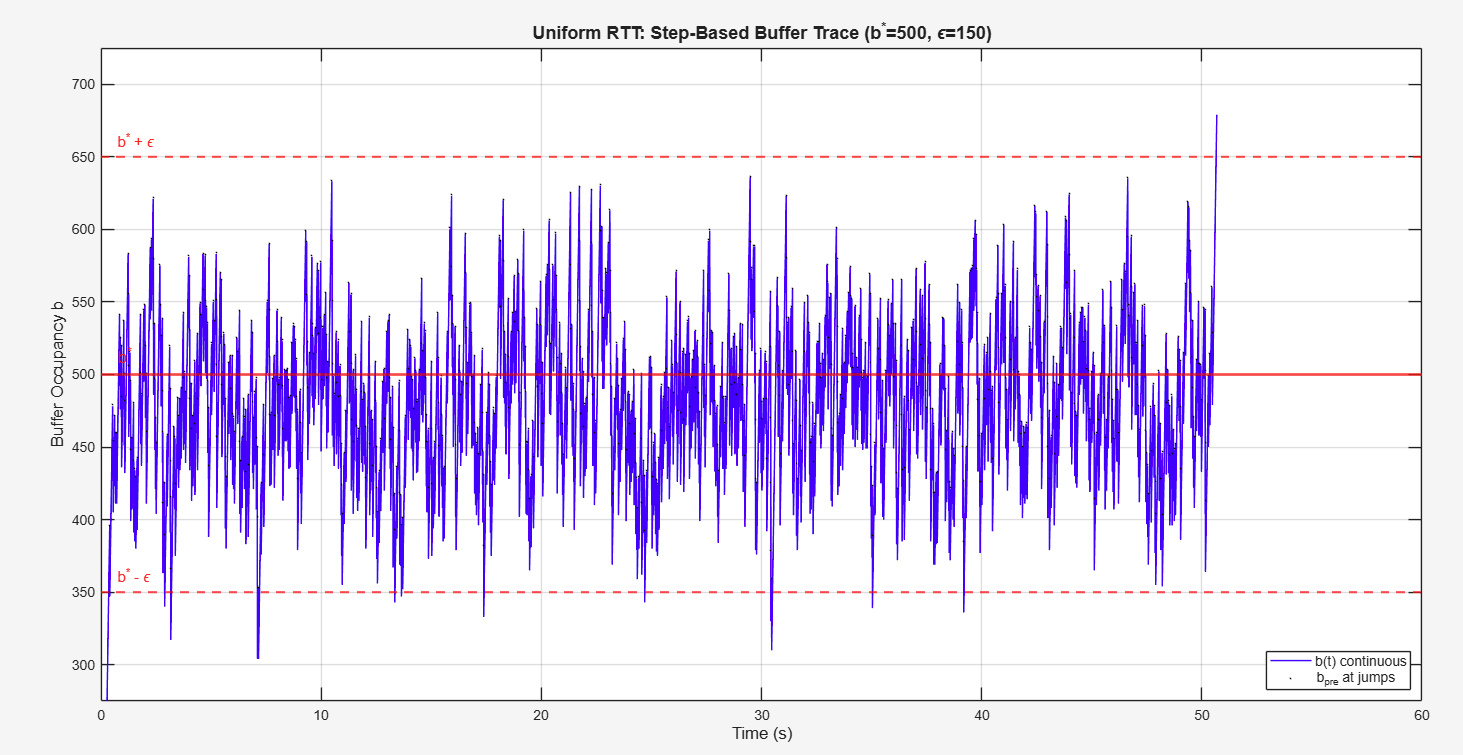
The buffer level is bounded in the range of \([b^* - \varepsilon, b^* + \varepsilon]\) as expected. Note that the stability result \(|b_j - b^*| \leq \varepsilon\) applies to the pre-drain buffer level (the state just before the jump executes). Immediately after the jump, the buffer drops by \(C_s\), so the post-drain level \(b_j^+ = b_j - C_s\) can be as low as \(r_{in}(\mu - \delta)\), which is \(C_s\) below the lower fence \(b^* - \varepsilon\). This is not a violation of stability — the system then fills continuously at rate \(r_{in}\) during the flow phase, and by the time the next ACK arrives, the pre-drain level is again within \([b^* - \varepsilon, b^* + \varepsilon]\).

A good way to validate the result is to purposely set RTT. In the following, I alternatively set the RTT to be always \(\mu - \delta\), \(\mu\), and \(\mu + \delta\) to see the result:

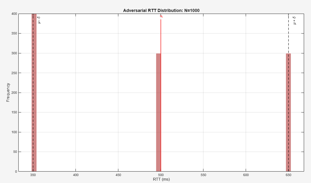
And as expected, the pre-drain buffer level is always bounded by \([b^* - \varepsilon, b^* + \varepsilon]\):

Exploration of the RTT distributions in the interval

Hardware Simulation Result:

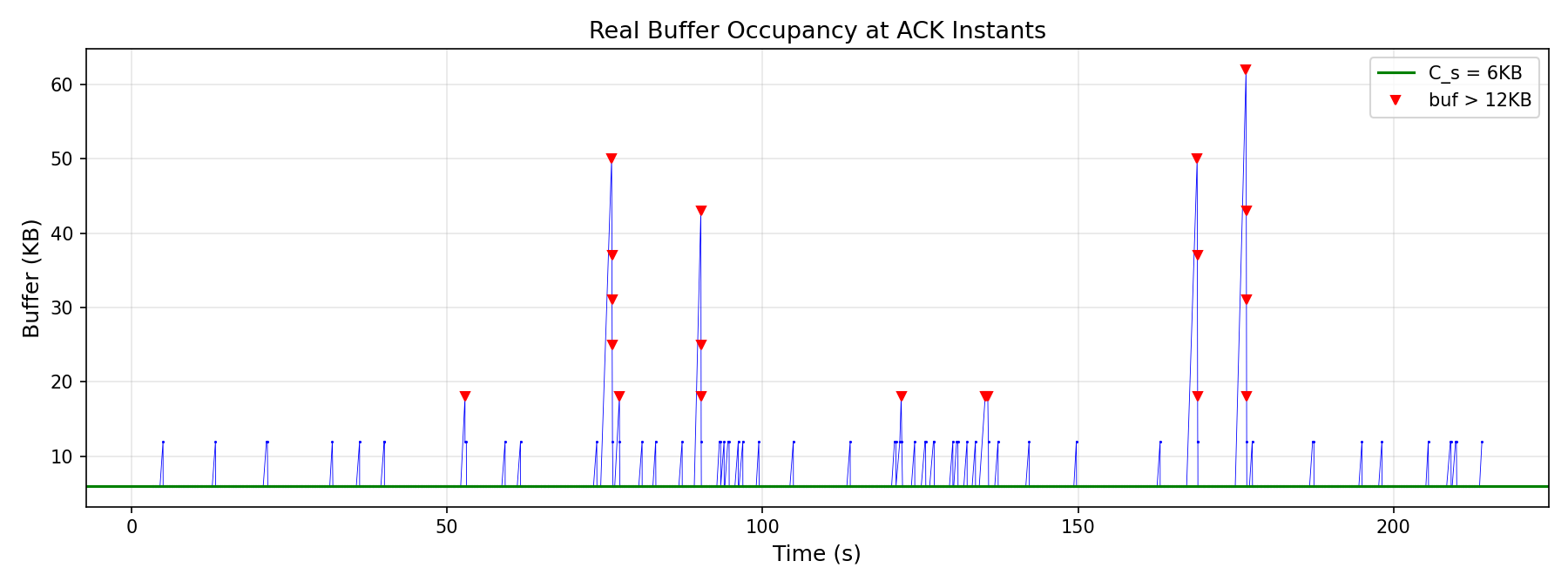
So in reality, I did not actually set the \(T_{max}\) here, and the period of network congestion really affects the result, as we can see a spike in the buffer level during network congestion. But most of the time, the buffer level is still bounded in the neighborhood of \(b^*\).

This is the plot of the real buffer occupancy level:

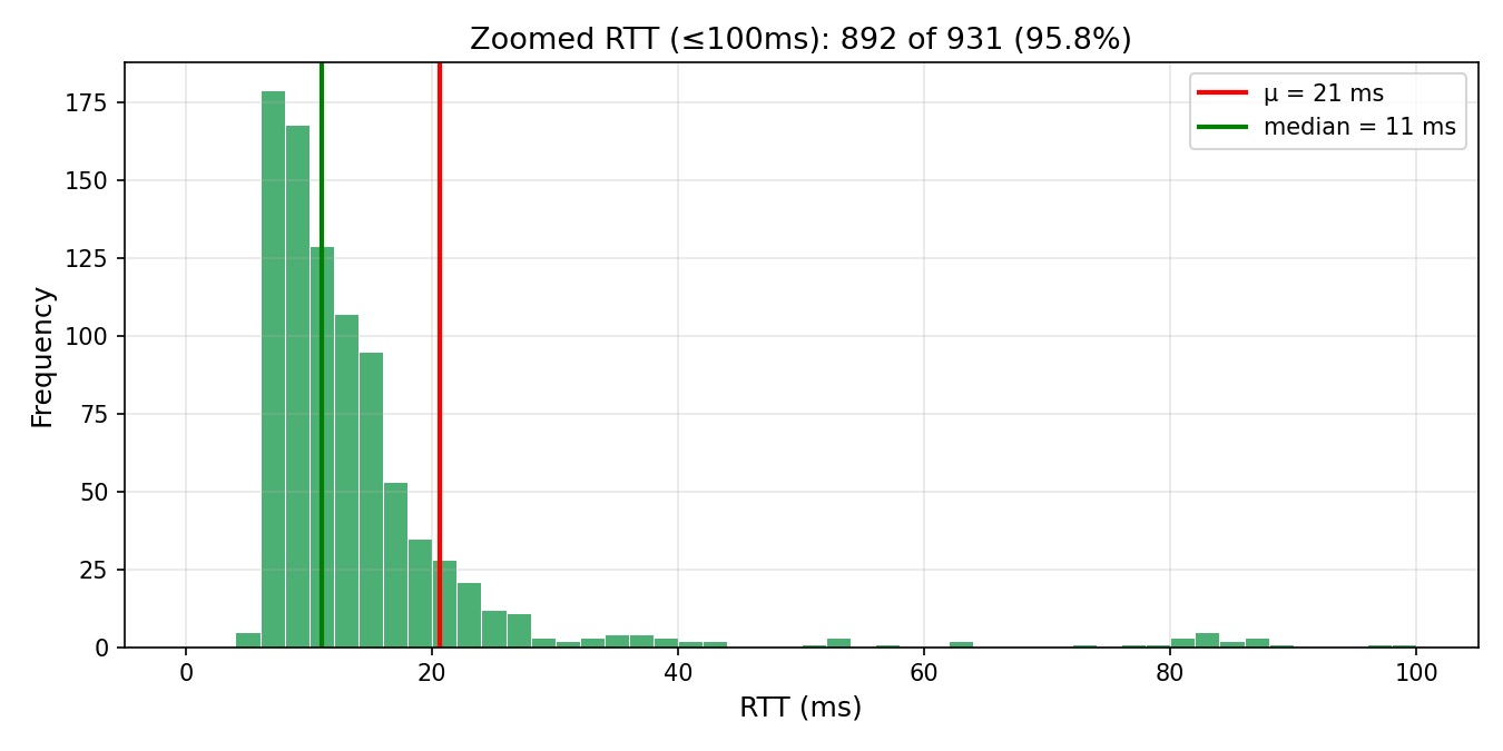
This is the histogram of the RTT. It is more like an exponential distribution, and heavily skewed to the right.

The Exponential Distribution Case

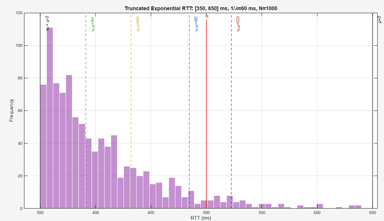
In the previous analysis, we only assumed that the RTT is bounded in the interval of \([\mu - \delta, \mu + \delta]\), but we can further assume that the \(RTT \sim \operatorname{Exponential}(\lambda)\), where \(\lambda\) is the rate parameter of the exponential distribution.

Similarly, it is truncated in the range \([\mu - \delta, \mu + \delta]\).

The PDF of the truncated exponential distribution where \(a = \mu - \delta\) and \(b = \mu + \delta\) is:

\[ f(x) = \frac{\lambda e^{-\lambda x}}{e^{-\lambda a} - e^{-\lambda b}} \quad \text{for } x \in [a, b] \]

The mean is given by

\[ E[RTT] = \int_{a}^{b} x f(x) dx \\ = a + \frac{1}{\lambda} - \frac{b - a}{e^{\lambda (b - a)} - 1} \]

Since \(L = b - a = 2\delta\) and \(a = \mu - \delta\), \(E[RTT] = (\mu - \delta) + \frac{1}{\lambda} - \frac{2\delta}{e^{2 \lambda \delta} - 1}\).

The CDF of the truncated exponential distribution is:

\[ F(x) = \frac{1 - e^{-\lambda (x - a)}}{1 - e^{-\lambda L}} \quad \text{for } x \in [a, b] \]

Let \(p\) be the desired confidence level, then we can find the confidence interval of the RTT by solving:

\[ p = F(x) = \frac{1 - e^{-\lambda (x - a)}}{1 - e^{-\lambda L}} \\ p(1 - e^{-\lambda L}) = 1 - e ^{-\lambda (x - a)} \\ e^{-\lambda (x-a)} = 1 - p(1 - e^{-\lambda L}) \\ x_p = a - \frac{1}{\lambda} \ln (1 - p (1 - e^{-\lambda L}))\]

For a confidence level of \(90\%\), take \(x_0\) and \(x_{0.9}\) to characterize the buffer range. Since the exponential distribution is right-skewed, we use a one-sided interval — the lower bound \(x_0 = a\) is the physical minimum (harmless), and all overflow risk is in the upper tail.

\[x_0 = a - \frac{1}{\lambda} \ln (1 - 0 (1 - e^{-\lambda L})) = a = \mu - \delta\]

\[x_{0.9} = a - \frac{1}{\lambda} \ln (1 - 0.9 (1 - e^{-\lambda L}))\]

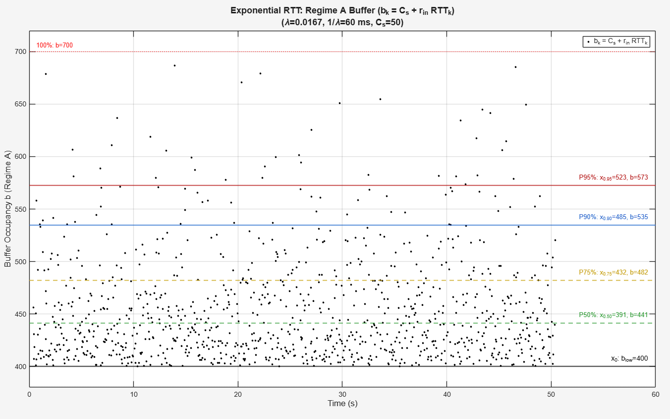
Therefore, with a confidence level of \(90\%\), \(b_j\) is bounded in the range \([C_s + r_{in} x_0, C_s + r_{in} x_{0.9}]\).

Simulation Result

Its RTT distribution:

Its buffer level:

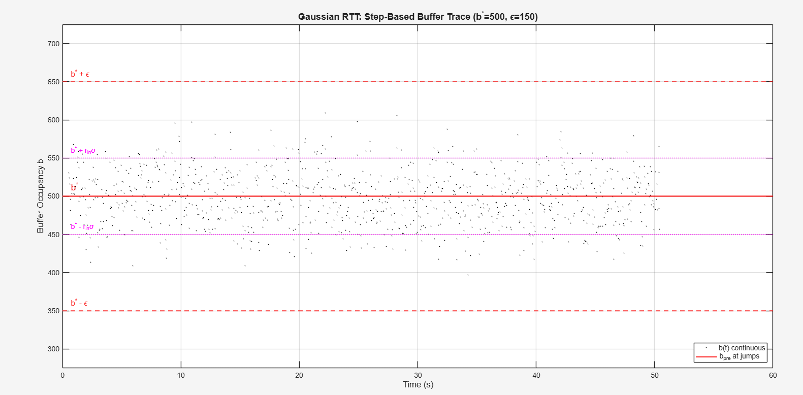
The Normal Distribution Case

In some cases, when the network is stable, the RTT distribution can be more like a normal distribution.

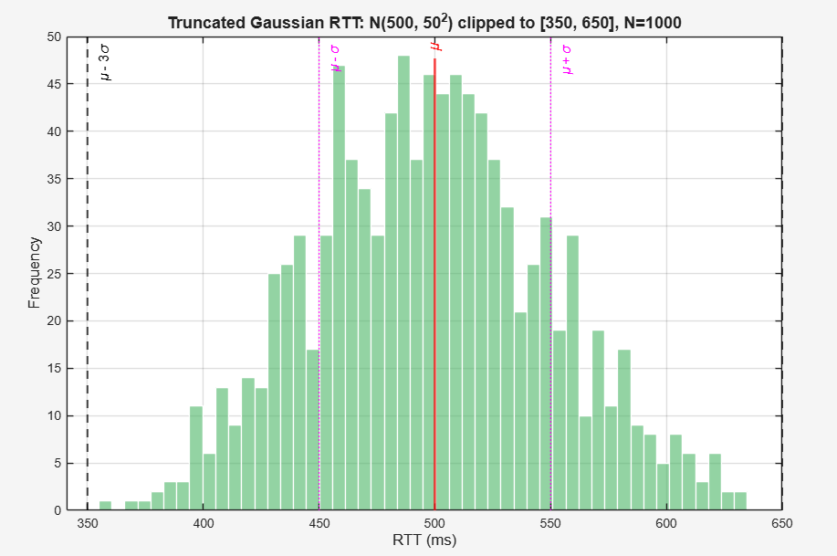
The buffer level:

Conclusion

Therefore, I have shown that the buffer level of the audio streaming process is uniformly globally practically stable (UGpS) in the neighborhood \(\mathcal{A}_\epsilon = \{b \in \mathbb{R} : |b - b^*| < \varepsilon\}\) of \(b^* = r_{in} \mu + C_s\) with a tolerance of \(\varepsilon = r_{in} \delta\), as long as the network RTT is bounded in the range \([\mu - \delta, \mu + \delta]\).

I also explored that, when the RTT distribution is exponential, we can further find the confidence interval of the RTT, therefore better characterize the buffer level distribution and find a more accurate max buffer size that is safe enough to use.

Works Cited

[1] S. Bohacek, J. P. Hespanha, J. Lee, and K. Obraczka, "Analysis of a TCP hybrid model," Tech. Rep., University of Southern California, 2001.

[2] Y.-C. Chan and H.-J. Lee, "A hybrid congestion control for TCP over high speed networks," in Proc. ICGEC, IEEE, 2012.

[3] G. Cofano, L. De Cicco, and S. Mascolo, "Characterizing adaptive video streaming control systems," in Proc. American Control Conference, 2015.

[4] W. Jiang and A. Seuret, "Improved stability analysis of networked control systems under asynchronous sampling and input delay," in Proc. IFAC NecSys Workshop, 2010.